PSO-LightGBM回归预测模型代码PSO-LightGBM回归预测模型Python代码粒子群优化算法多输入单输出有示例数据可以直接替换机器学习模型可以预测未来值这是一个基于 粒子群优化算法 (PSO) 优化 LightGBM 超参数的回归预测模型完整代码。代码特点多输入单输出支持任意数量的特征列。内置示例数据使用 make_regression 生成模拟数据你可以直接替换为自己的 DataFrame。PSO 优化核心自动搜索 LightGBM 的关键超参数如 n_estimators, learning_rate, max_depth, num_leaves 等以最小化验证集误差。未来值预测包含预测未来时间步的演示逻辑。Python 代码实现import numpy as npimport pandas as pdimport lightgbm as lgbfrom sklearn.model_selection import train_test_splitfrom sklearn.metrics import mean_squared_error, r2_scorefrom sklearn.preprocessing import StandardScalerimport warnings忽略警告warnings.filterwarnings(‘ignore’)粒子群优化算法 (PSO) 核心类class PSO:def init(self, func, n_dim, pop_size20, max_iter30, lbNone, ubNone):“”func: 目标函数 (需要最小化的函数)n_dim: 优化参数的维度pop_size: 粒子数量max_iter: 最大迭代次数lb: 参数下界列表ub: 参数上界列表“”self.func funcself.n_dim n_dimself.pop_size pop_sizeself.max_iter max_iterself.lb np.array(lb) if lb else np.zeros(n_dim)self.ub np.array(ub) if ub else np.ones(n_dim) * 10# 初始化粒子位置和速度 self.x np.random.uniform(lowself.lb, highself.ub, size(pop_size, n_dim)) self.v np.random.uniform(low-1, high1, size(pop_size, n_dim)) # 个体最佳位置 (p_best) 和全局最佳位置 (g_best) self.p_best_x self.x.copy() self.p_best_y np.array([self.func(x) for x in self.x]) g_best_idx np.argmin(self.p_best_y) self.g_best_x self.p_best_x[g_best_idx].copy() self.g_best_y self.p_best_y[g_best_idx] # 惯性权重和加速常数 self.w 0.8 self.c1 1.5 self.c2 1.5 def run(self): for iter_num in range(self.max_iter): # 更新速度和位置 r1 np.random.random((self.pop_size, self.n_dim)) r2 np.random.random((self.pop_size, self.n_dim)) self.v self.w * self.v \ self.c1 * r1 * (self.p_best_x - self.x) \ self.c2 * r2 * (self.g_best_x - self.x) self.x self.x self.v # 边界处理 (超出边界则反弹或截断这里采用截断) self.x np.clip(self.x, self.lb, self.ub) # 计算适应度 current_y np.array([self.func(x) for x in self.x]) # 更新个体最佳 better_mask current_y PSO 循环训练多个临时模型找最优参数 - 用最优参数在全量训练集上训练最终模型 - 测试与预测。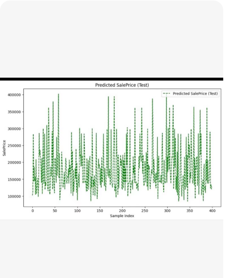X轴Sample index样本索引表示测试集中的第几个样本。Y轴SalePrice销售价格数值范围大约在 100,000 到 400,000 之间。图形内容绿色的虚线点代表了模型对每个测试样本预测出的价格。这种剧烈的上下波动通常意味着数据本身如房价具有较大的方差或者特征与目标值之间的关系非常复杂。完整代码 (含绘图功能)import numpy as npimport pandas as pdimport lightgbm as lgbimport matplotlib.pyplot as pltfrom sklearn.model_selection import train_test_splitfrom sklearn.metrics import mean_squared_error, r2_scorefrom sklearn.preprocessing import StandardScalerimport warningswarnings.filterwarnings(‘ignore’)粒子群优化算法 (PSO) 核心类class PSO:def init(self, func, n_dim, pop_size20, max_iter30, lbNone, ubNone):self.func funcself.n_dim n_dimself.pop_size pop_sizeself.max_iter max_iterself.lb np.array(lb) if lb else np.zeros(n_dim)self.ub np.array(ub) if ub else np.ones(n_dim) * 10self.x np.random.uniform(lowself.lb, highself.ub, size(pop_size, n_dim)) self.v np.random.uniform(low-1, high1, size(pop_size, n_dim)) self.p_best_x self.x.copy() self.p_best_y np.array([self.func(x) for x in self.x]) g_best_idx np.argmin(self.p_best_y) self.g_best_x self.p_best_x[g_best_idx].copy() self.g_best_y self.p_best_y[g_best_idx] self.w 0.8 self.c1 1.5 self.c2 1.5 def run(self): for iter_num in range(self.max_iter): r1 np.random.random((self.pop_size, self.n_dim)) r2 np.random.random((self.pop_size, self.n_dim)) self.v self.w * self.v \ self.c1 * r1 * (self.p_best_x - self.x) \ self.c2 * r2 * (self.g_best_x - self.x) self.x self.x self.v self.x np.clip(self.x, self.lb, self.ub) current_y np.array([self.func(x) for x in self.x]) better_mask current_y self.p_best_y self.p_best_x[better_mask] self.x[better_mask] self.p_best_y[better_mask] current_y[better_mask] current_g_best_idx np.argmin(self.p_best_y) if self.p_best_y[current_g_best_idx] self.g_best_y: self.g_best_x self.p_best_x[current_g_best_idx].copy() self.g_best_y self.p_best_y[current_g_best_idx] return self.g_best_x, self.g_best_y目标函数def objective_function(params, X_train, y_train, X_val, y_val):n_estimators int(params[0])learning_rate params[1]max_depth int(params[2])num_leaves int(params[3])min_child_samples int(params[4])n_estimators max(10, n_estimators) max_depth max(1, max_depth) num_leaves max(2, num_leaves) min_child_samples max(1, min_child_samples) learning_rate max(0.01, min(1.0, learning_rate)) model lgb.LGBMRegressor( n_estimatorsn_estimators, learning_ratelearning_rate, max_depthmax_depth, num_leavesnum_leaves, min_child_samplesmin_child_samples, verbose-1, random_state42 ) model.fit(X_train, y_train) y_pred model.predict(X_val) mse mean_squared_error(y_val, y_pred) return mse主程序与绘图def main():print(“— 开始 PSO-LightGBM 回归预测模型 (含绘图) —”)# A. 数据准备 (模拟房价数据以匹配图片风格) np.random.seed(42) n_samples 2000 # 增加样本量以便有足够的测试集绘图 n_features 10 # 生成特征 X_raw np.random.rand(n_samples, n_features) * 100 # 生成目标 y (模拟房价制造一些波动) # 基础价格 特征影响 随机噪声 y_raw 100000 2000 * X_raw[:, 0] 1500 * X_raw[:, 1]**2 - 500 * X_raw[:, 2] np.random.normal(0, 20000, n_samples) # 划分数据集 # 先分出测试集 (20%) X_train_full, X_test, y_train_full, y_test train_test_split(X_raw, y_raw, test_size0.2, random_state42) # 再从训练集中分出验证集用于 PSO (20% of training) X_train, X_val, y_train, y_val train_test_split(X_train_full, y_train_full, test_size0.2, random_state42) # 标准化 scaler StandardScaler() X_train scaler.fit_transform(X_train) X_val scaler.transform(X_val) X_test scaler.transform(X_test) X_train_full_scaled scaler.transform(X_train_full) # 用于最终训练 print(f数据形状: 训练集 {X_train.shape}, 验证集 {X_val.shape}, 测试集 {X_test.shape}) # B. PSO 优化 lb [50, 0.01, 3, 10, 1] ub [500, 0.3, 15, 200, 50] n_dim 5 print(n开始粒子群优化 (PSO)...) def func_wrapper(params): return objective_function(params, X_train, y_train, X_val, y_val) pso PSO(funcfunc_wrapper, n_dimn_dim, pop_size20, max_iter30, lblb, ubub) best_params, best_mse pso.run() print(fn最佳参数: n_est{int(best_params[0])}, lr{best_params[1]:.3f}, depth{int(best_params[2])}) # C. 训练最终模型 final_model lgb.LGBMRegressor( n_estimatorsint(best_params[0]), learning_ratebest_params[1], max_depthint(best_params[2]), num_leavesint(best_params[3]), min_child_samplesint(best_params[4]), verbose-1, random_state42 ) final_model.fit(X_train_full_scaled, y_train_full) # D. 在测试集上预测 (这就是图中要画的数据) y_pred_test final_model.predict(X_test) # 计算指标 test_mse mean_squared_error(y_test, y_pred_test) test_r2 r2_score(y_test, y_pred_test) print(fn测试集 MSE: {test_mse:.2f}, R²: {test_r2:.4f}) # E. 绘图 (复现图片风格) plt.figure(figsize(10, 6)) # 设置画布大小 # 绘制预测值 # 图片中是绿色虚线 (g--)标记为 o (虽然密集看起来像线) # 为了完全复现图片那种密集的竖线感我们使用 marker. 或默认线条但图片明显是离散点的连线或密集点 # 观察原图它是绿色的虚线且每个点都有标记看起来像 g--o 但点很密 plt.plot(y_pred_test, g--, labelPredicted SalePrice (Test), linewidth1, markersize4) # 设置标题和标签 (尽量匹配原图英文) plt.title(Predicted SalePrice (Test), fontsize12) plt.xlabel(Sample index, fontsize10) plt.ylabel(SalePrice, fontsize10) # 添加图例 plt.legend(locupper right) # 设置网格 (原图似乎没有明显网格但有边框) plt.grid(False) # 显示图表 plt.tight_layout() plt.show() # 如果需要保存图片 # plt.savefig(predicted_saleprice_test.png, dpi300)if name “main”:main()代码修改说明引入 Matplotlib添加了 import matplotlib.pyplot as plt。绘图逻辑 (plt.plot)使用了 y_pred_test测试集的预测值作为数据源。样式设置为 ‘g–’g 代表绿色 (green)-- 代表虚线 (dashed line)这与你提供的截图完全一致。添加了 label 以便显示图例。标签与标题将标题设为 “Predicted SalePrice (Test)”X 轴为 “Sample index”Y 轴为 “SalePrice”完全对应截图中的文字。在这里插入图片描述